# Unfiltered human PBMCs (10X Genomics)

<script>
document.addEventListener("click", function (event) {
    if (event.target.classList.contains("rebook-collapse")) {
        event.target.classList.toggle("active");
        var content = event.target.nextElementSibling;
        if (content.style.display === "block") {
            content.style.display = "none";
        } else {
            content.style.display = "block";
        }
    }
})
</script>

<style>
.rebook-collapse {
  background-color: #eee;
  color: #444;
  cursor: pointer;
  padding: 18px;
  width: 100%;
  border: none;
  text-align: left;
  outline: none;
  font-size: 15px;
}

.rebook-content {
  padding: 0 18px;
  display: none;
  overflow: hidden;
  background-color: #f1f1f1;
}
</style>

## Introduction

Here, we describe a brief analysis of the peripheral blood mononuclear cell (PBMC) dataset from 10X Genomics [@zheng2017massively].
The data are publicly available from the [10X Genomics website](https://support.10xgenomics.com/single-cell-gene-expression/datasets/2.1.0/pbmc4k),
from which we download the raw gene/barcode count matrices, i.e., before cell calling from the _CellRanger_ pipeline.

## Data loading


```r
library(DropletTestFiles)
raw.path <- getTestFile("tenx-2.1.0-pbmc4k/1.0.0/raw.tar.gz")
out.path <- file.path(tempdir(), "pbmc4k")
untar(raw.path, exdir=out.path)

library(DropletUtils)
fname <- file.path(out.path, "raw_gene_bc_matrices/GRCh38")
sce.pbmc <- read10xCounts(fname, col.names=TRUE)
```


```r
library(scater)
rownames(sce.pbmc) <- uniquifyFeatureNames(
    rowData(sce.pbmc)$ID, rowData(sce.pbmc)$Symbol)

library(EnsDb.Hsapiens.v86)
location <- mapIds(EnsDb.Hsapiens.v86, keys=rowData(sce.pbmc)$ID, 
    column="SEQNAME", keytype="GENEID")
```

## Quality control

We perform cell detection using the `emptyDrops()` algorithm, as discussed in [Advanced Section 7.2](http://bioconductor.org/books/3.19/OSCA.advanced/droplet-processing.html#qc-droplets).


```r
set.seed(100)
e.out <- emptyDrops(counts(sce.pbmc))
sce.pbmc <- sce.pbmc[,which(e.out$FDR <= 0.001)]
```


```r
unfiltered <- sce.pbmc
```

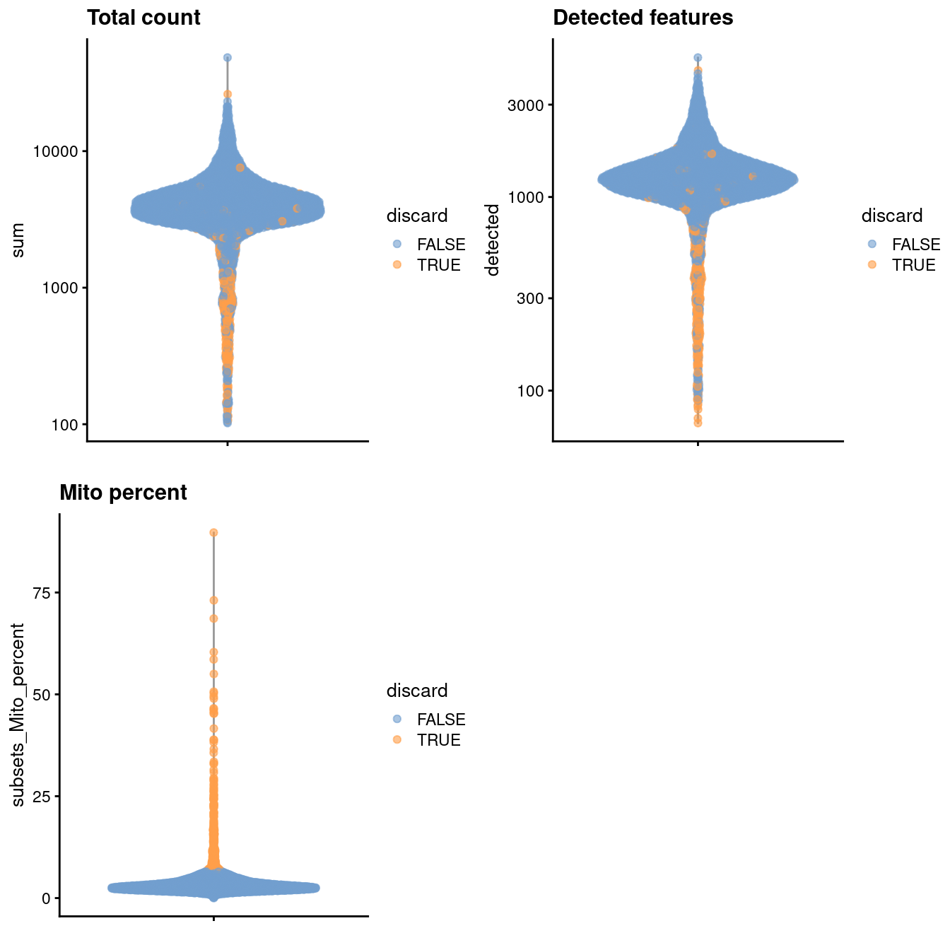
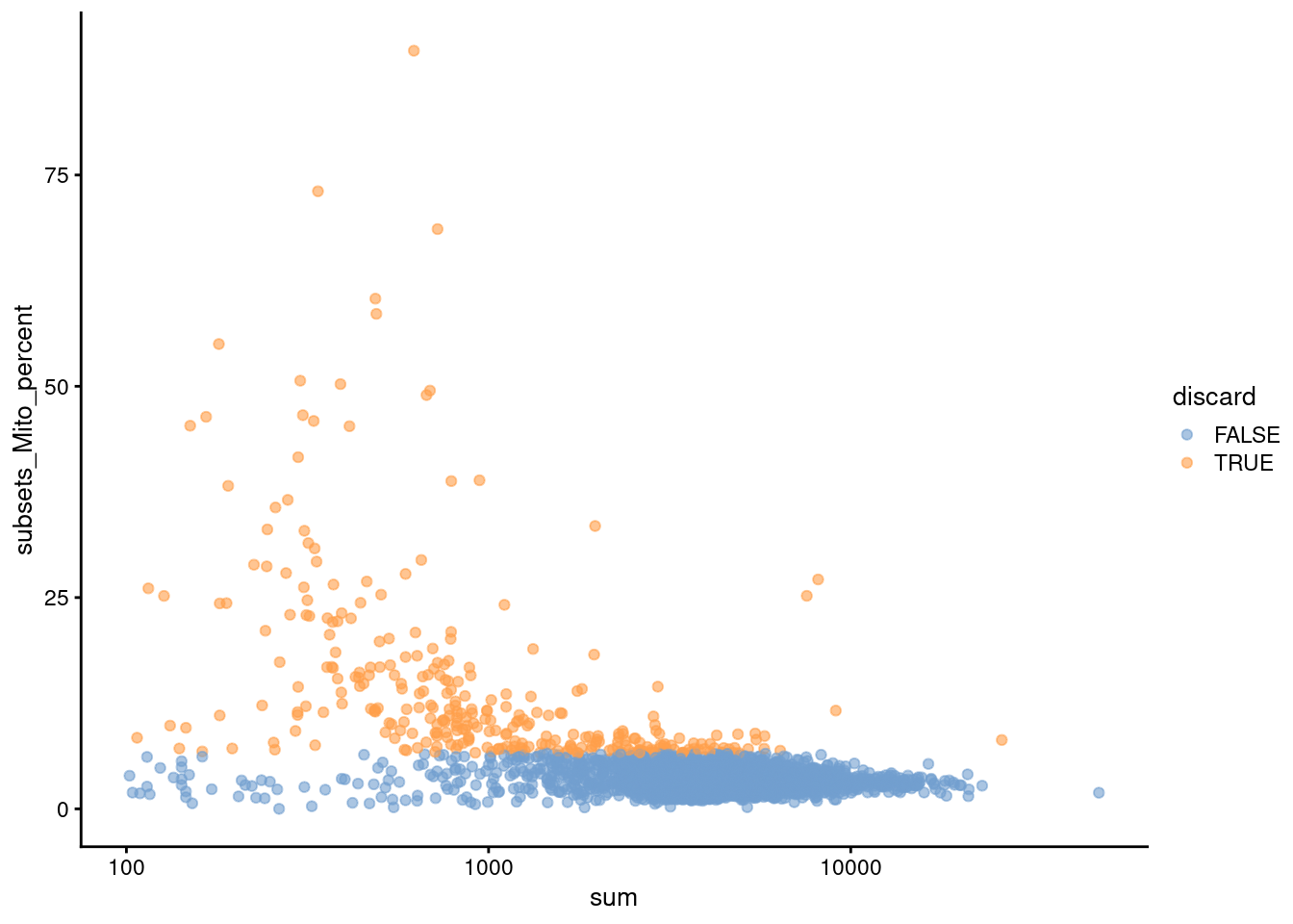
We use a relaxed QC strategy and only remove cells with large mitochondrial proportions, using it as a proxy for cell damage.
This reduces the risk of removing cell types with low RNA content, especially in a heterogeneous PBMC population with many different cell types.


```r
stats <- perCellQCMetrics(sce.pbmc, subsets=list(Mito=which(location=="MT")))
high.mito <- isOutlier(stats$subsets_Mito_percent, type="higher")
sce.pbmc <- sce.pbmc[,!high.mito]
```


```r
summary(high.mito)
```

```
##    Mode   FALSE    TRUE 
## logical    3985     315
```


```r
colData(unfiltered) <- cbind(colData(unfiltered), stats)
unfiltered$discard <- high.mito

gridExtra::grid.arrange(
    plotColData(unfiltered, y="sum", colour_by="discard") +
        scale_y_log10() + ggtitle("Total count"),
    plotColData(unfiltered, y="detected", colour_by="discard") +
        scale_y_log10() + ggtitle("Detected features"),
    plotColData(unfiltered, y="subsets_Mito_percent",
        colour_by="discard") + ggtitle("Mito percent"),
    ncol=2
)
```

<div class="figure">
<img src="tenx-unfiltered-pbmc4k_files/figure-html/unref-unfiltered-pbmc-qc-1.png" alt="Distribution of various QC metrics in the PBMC dataset after cell calling. Each point is a cell and is colored according to whether it was discarded by the mitochondrial filter." width="672" />
<p class="caption">(\#fig:unref-unfiltered-pbmc-qc)Distribution of various QC metrics in the PBMC dataset after cell calling. Each point is a cell and is colored according to whether it was discarded by the mitochondrial filter.</p>
</div>


```r
plotColData(unfiltered, x="sum", y="subsets_Mito_percent",
    colour_by="discard") + scale_x_log10()
```

<div class="figure">
<img src="tenx-unfiltered-pbmc4k_files/figure-html/unref-unfiltered-pbmc-mito-1.png" alt="Proportion of mitochondrial reads in each cell of the PBMC dataset compared to its total count." width="672" />
<p class="caption">(\#fig:unref-unfiltered-pbmc-mito)Proportion of mitochondrial reads in each cell of the PBMC dataset compared to its total count.</p>
</div>

## Normalization


```r
library(scran)
set.seed(1000)
clusters <- quickCluster(sce.pbmc)
sce.pbmc <- computeSumFactors(sce.pbmc, cluster=clusters)
sce.pbmc <- logNormCounts(sce.pbmc)
```


```r
summary(sizeFactors(sce.pbmc))
```

```
##    Min. 1st Qu.  Median    Mean 3rd Qu.    Max. 
##   0.007   0.712   0.875   1.000   1.099  12.254
```


```r
plot(librarySizeFactors(sce.pbmc), sizeFactors(sce.pbmc), pch=16,
    xlab="Library size factors", ylab="Deconvolution factors", log="xy")
```

<div class="figure">
<img src="tenx-unfiltered-pbmc4k_files/figure-html/unref-unfiltered-pbmc-norm-1.png" alt="Relationship between the library size factors and the deconvolution size factors in the PBMC dataset." width="672" />
<p class="caption">(\#fig:unref-unfiltered-pbmc-norm)Relationship between the library size factors and the deconvolution size factors in the PBMC dataset.</p>
</div>

## Variance modelling


```r
set.seed(1001)
dec.pbmc <- modelGeneVarByPoisson(sce.pbmc)
top.pbmc <- getTopHVGs(dec.pbmc, prop=0.1)
```


```r
plot(dec.pbmc$mean, dec.pbmc$total, pch=16, cex=0.5,
    xlab="Mean of log-expression", ylab="Variance of log-expression")
curfit <- metadata(dec.pbmc)
curve(curfit$trend(x), col='dodgerblue', add=TRUE, lwd=2)
```

<div class="figure">
<img src="tenx-unfiltered-pbmc4k_files/figure-html/unref-unfiltered-pbmc-var-1.png" alt="Per-gene variance as a function of the mean for the log-expression values in the PBMC dataset. Each point represents a gene (black) with the mean-variance trend (blue) fitted to simulated Poisson counts." width="672" />
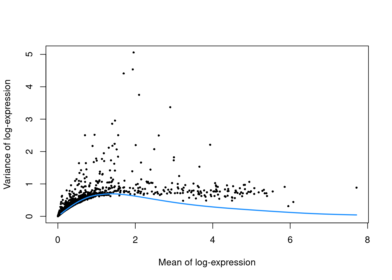
<p class="caption">(\#fig:unref-unfiltered-pbmc-var)Per-gene variance as a function of the mean for the log-expression values in the PBMC dataset. Each point represents a gene (black) with the mean-variance trend (blue) fitted to simulated Poisson counts.</p>
</div>

## Dimensionality reduction


```r
set.seed(10000)
sce.pbmc <- denoisePCA(sce.pbmc, subset.row=top.pbmc, technical=dec.pbmc)

set.seed(100000)
sce.pbmc <- runTSNE(sce.pbmc, dimred="PCA")

set.seed(1000000)
sce.pbmc <- runUMAP(sce.pbmc, dimred="PCA")
```

We verify that a reasonable number of PCs is retained.


```r
ncol(reducedDim(sce.pbmc, "PCA"))
```

```
## [1] 9
```

## Clustering


```r
g <- buildSNNGraph(sce.pbmc, k=10, use.dimred = 'PCA')
clust <- igraph::cluster_walktrap(g)$membership
colLabels(sce.pbmc) <- factor(clust)
```


```r
table(colLabels(sce.pbmc))
```

```
## 
##   1   2   3   4   5   6   7   8   9  10  11  12  13  14  15 
## 205 731 617  56 541 352 125  46 819  47 153  61 129  87  16
```


```r
plotTSNE(sce.pbmc, colour_by="label")
```

<div class="figure">
<img src="tenx-unfiltered-pbmc4k_files/figure-html/unref-unfiltered-pbmc-tsne-1.png" alt="Obligatory $t$-SNE plot of the PBMC dataset, where each point represents a cell and is colored according to the assigned cluster." width="672" />
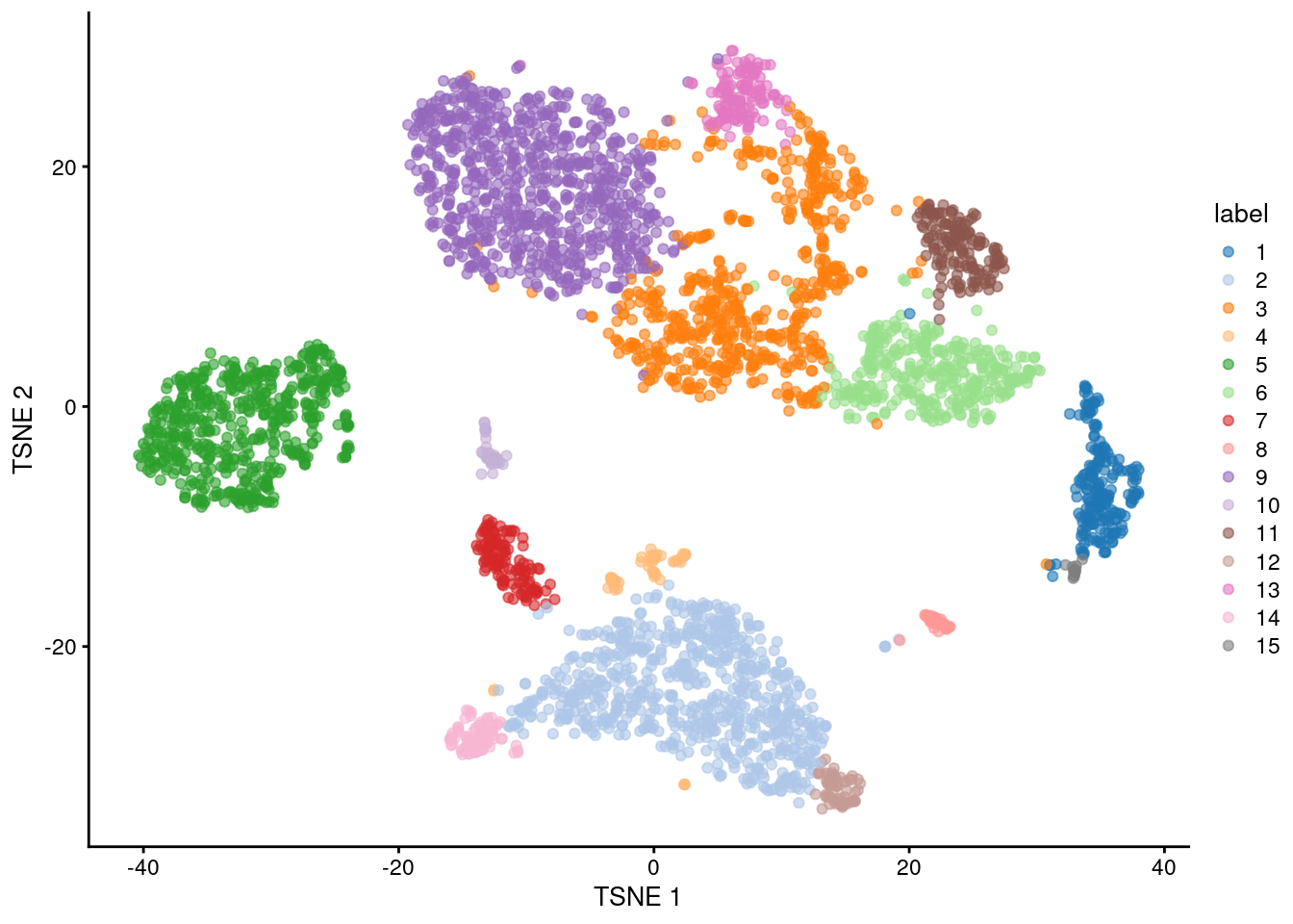
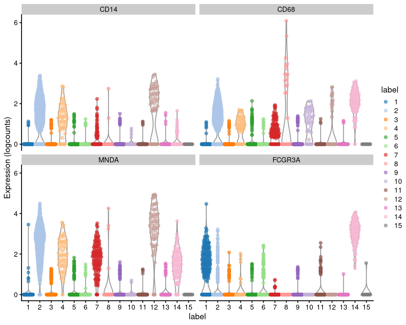
<p class="caption">(\#fig:unref-unfiltered-pbmc-tsne)Obligatory $t$-SNE plot of the PBMC dataset, where each point represents a cell and is colored according to the assigned cluster.</p>
</div>

## Interpretation




```r
markers <- findMarkers(sce.pbmc, pval.type="some", direction="up")
```

We examine the markers for cluster 2 in more detail.
High expression of _CD14_, _CD68_ and _MNDA_ combined with low expression of _FCGR3A_ (_CD16_) suggests that this cluster contains monocytes,
compared to macrophages in cluster 14 (Figure \@ref(fig:unref-mono-pbmc-markers)).


```r
marker.set <- markers[["2"]]
as.data.frame(marker.set[1:30,1:3])
```

```
##                  p.value        FDR summary.logFC
## MNDA           0.000e+00  0.000e+00        2.4270
## CSTA           0.000e+00 8.108e-321        2.2749
## FCN1          5.675e-266 6.374e-262        2.7085
## RP11-1143G9.4 4.422e-252 3.725e-248        2.6287
## VCAN          9.765e-235 6.581e-231        1.8445
## MS4A6A        2.287e-209 1.284e-205        1.5333
## FGL2          1.077e-208 5.183e-205        1.4499
## S100A12       3.976e-207 1.674e-203        2.4102
## LGALS2        1.732e-194 6.482e-191        2.0107
## CFD           1.207e-193 4.067e-190        1.4583
## AIF1          1.362e-180 4.173e-177        2.6862
## CD14          4.650e-170 1.306e-166        1.3215
## CLEC7A        3.055e-169 7.917e-166        1.0966
## TYMP          4.932e-166 1.187e-162        2.0425
## CD68          1.008e-161 2.264e-158        1.1025
## S100A8        2.499e-158 5.262e-155        4.5407
## SERPINA1      1.262e-157 2.502e-154        1.5040
## TNFSF13B      3.069e-151 5.745e-148        1.0353
## KLF4          1.351e-150 2.395e-147        1.2414
## AP1S2         3.613e-149 6.087e-146        1.8689
## CFP           8.387e-144 1.346e-140        1.1019
## S100A9        1.301e-141 1.993e-138        4.5307
## NAMPT         1.074e-138 1.573e-135        1.1066
## IFI30         2.558e-133 3.591e-130        0.9717
## MPEG1         9.448e-132 1.273e-128        0.9856
## CYBB          5.226e-129 6.773e-126        1.1825
## LGALS3        2.868e-128 3.580e-125        0.9434
## LYZ           1.108e-123 1.334e-120        5.0812
## CPVL          3.905e-123 4.537e-120        0.8642
## CD36          6.119e-123 6.873e-120        0.9696
```




```r
plotExpression(sce.pbmc, features=c("CD14", "CD68",
    "MNDA", "FCGR3A"), x="label", colour_by="label")
```

<div class="figure">
<img src="tenx-unfiltered-pbmc4k_files/figure-html/unref-mono-pbmc-markers-1.png" alt="Distribution of expression values for monocyte and macrophage markers across clusters in the PBMC dataset." width="672" />
<p class="caption">(\#fig:unref-mono-pbmc-markers)Distribution of expression values for monocyte and macrophage markers across clusters in the PBMC dataset.</p>
</div>

## Session Info {-}

<button class="rebook-collapse">View session info</button>
<div class="rebook-content">
```
R version 4.4.0 beta (2024-04-15 r86425)
Platform: x86_64-pc-linux-gnu
Running under: Ubuntu 22.04.4 LTS

Matrix products: default
BLAS:   /home/biocbuild/bbs-3.19-bioc/R/lib/libRblas.so 
LAPACK: /usr/lib/x86_64-linux-gnu/lapack/liblapack.so.3.10.0

locale:
 [1] LC_CTYPE=en_US.UTF-8       LC_NUMERIC=C              
 [3] LC_TIME=en_GB              LC_COLLATE=C              
 [5] LC_MONETARY=en_US.UTF-8    LC_MESSAGES=en_US.UTF-8   
 [7] LC_PAPER=en_US.UTF-8       LC_NAME=C                 
 [9] LC_ADDRESS=C               LC_TELEPHONE=C            
[11] LC_MEASUREMENT=en_US.UTF-8 LC_IDENTIFICATION=C       

time zone: America/New_York
tzcode source: system (glibc)

attached base packages:
[1] stats4    stats     graphics  grDevices utils     datasets  methods  
[8] base     

other attached packages:
 [1] scran_1.32.0                EnsDb.Hsapiens.v86_2.99.0  
 [3] ensembldb_2.28.0            AnnotationFilter_1.28.0    
 [5] GenomicFeatures_1.56.0      AnnotationDbi_1.66.0       
 [7] scater_1.32.0               ggplot2_3.5.1              
 [9] scuttle_1.14.0              DropletUtils_1.24.0        
[11] SingleCellExperiment_1.26.0 SummarizedExperiment_1.34.0
[13] Biobase_2.64.0              GenomicRanges_1.56.0       
[15] GenomeInfoDb_1.40.0         IRanges_2.38.0             
[17] S4Vectors_0.42.0            BiocGenerics_0.50.0        
[19] MatrixGenerics_1.16.0       matrixStats_1.3.0          
[21] DropletTestFiles_1.14.0     BiocStyle_2.32.0           
[23] rebook_1.14.0              

loaded via a namespace (and not attached):
  [1] jsonlite_1.8.8            CodeDepends_0.6.6        
  [3] magrittr_2.0.3            ggbeeswarm_0.7.2         
  [5] farver_2.1.1              rmarkdown_2.26           
  [7] BiocIO_1.14.0             zlibbioc_1.50.0          
  [9] vctrs_0.6.5               memoise_2.0.1            
 [11] Rsamtools_2.20.0          DelayedMatrixStats_1.26.0
 [13] RCurl_1.98-1.14           htmltools_0.5.8.1        
 [15] S4Arrays_1.4.0            AnnotationHub_3.12.0     
 [17] curl_5.2.1                BiocNeighbors_1.22.0     
 [19] Rhdf5lib_1.26.0           SparseArray_1.4.0        
 [21] rhdf5_2.48.0              sass_0.4.9               
 [23] bslib_0.7.0               cachem_1.0.8             
 [25] GenomicAlignments_1.40.0  igraph_2.0.3             
 [27] mime_0.12                 lifecycle_1.0.4          
 [29] pkgconfig_2.0.3           rsvd_1.0.5               
 [31] Matrix_1.7-0              R6_2.5.1                 
 [33] fastmap_1.1.1             GenomeInfoDbData_1.2.12  
 [35] digest_0.6.35             colorspace_2.1-0         
 [37] dqrng_0.3.2               irlba_2.3.5.1            
 [39] ExperimentHub_2.12.0      RSQLite_2.3.6            
 [41] beachmat_2.20.0           labeling_0.4.3           
 [43] filelock_1.0.3            fansi_1.0.6              
 [45] httr_1.4.7                abind_1.4-5              
 [47] compiler_4.4.0            bit64_4.0.5              
 [49] withr_3.0.0               BiocParallel_1.38.0      
 [51] viridis_0.6.5             DBI_1.2.2                
 [53] highr_0.10                HDF5Array_1.32.0         
 [55] R.utils_2.12.3            rappdirs_0.3.3           
 [57] DelayedArray_0.30.0       bluster_1.14.0           
 [59] rjson_0.2.21              tools_4.4.0              
 [61] vipor_0.4.7               beeswarm_0.4.0           
 [63] R.oo_1.26.0               glue_1.7.0               
 [65] restfulr_0.0.15           rhdf5filters_1.16.0      
 [67] grid_4.4.0                Rtsne_0.17               
 [69] cluster_2.1.6             generics_0.1.3           
 [71] gtable_0.3.5              R.methodsS3_1.8.2        
 [73] metapod_1.12.0            BiocSingular_1.20.0      
 [75] ScaledMatrix_1.12.0       utf8_1.2.4               
 [77] XVector_0.44.0            ggrepel_0.9.5            
 [79] BiocVersion_3.19.1        pillar_1.9.0             
 [81] limma_3.60.0              dplyr_1.1.4              
 [83] BiocFileCache_2.12.0      lattice_0.22-6           
 [85] FNN_1.1.4                 rtracklayer_1.64.0       
 [87] bit_4.0.5                 tidyselect_1.2.1         
 [89] locfit_1.5-9.9            Biostrings_2.72.0        
 [91] knitr_1.46                gridExtra_2.3            
 [93] bookdown_0.39             ProtGenerics_1.36.0      
 [95] edgeR_4.2.0               xfun_0.43                
 [97] statmod_1.5.0             UCSC.utils_1.0.0         
 [99] lazyeval_0.2.2            yaml_2.3.8               
[101] evaluate_0.23             codetools_0.2-20         
[103] tibble_3.2.1              BiocManager_1.30.22      
[105] graph_1.82.0              cli_3.6.2                
[107] uwot_0.2.2                munsell_0.5.1            
[109] jquerylib_0.1.4           Rcpp_1.0.12              
[111] dir.expiry_1.12.0         dbplyr_2.5.0             
[113] png_0.1-8                 XML_3.99-0.16.1          
[115] parallel_4.4.0            blob_1.2.4               
[117] sparseMatrixStats_1.16.0  bitops_1.0-7             
[119] viridisLite_0.4.2         scales_1.3.0             
[121] purrr_1.0.2               crayon_1.5.2             
[123] rlang_1.1.3               cowplot_1.1.3            
[125] KEGGREST_1.44.0          
```
</div>