# Grun human pancreas (CEL-seq2) ## Introduction This workflow performs an analysis of the @grun2016denovo CEL-seq2 dataset consisting of human pancreas cells from various donors. ## Data loading ```r library(scRNAseq) sce.grun <- GrunPancreasData() ``` We convert to Ensembl identifiers, and we remove duplicated genes or genes without Ensembl IDs. ```r library(org.Hs.eg.db) gene.ids <- mapIds(org.Hs.eg.db, keys=rowData(sce.grun)$symbol, keytype="SYMBOL", column="ENSEMBL") keep <- !is.na(gene.ids) & !duplicated(gene.ids) sce.grun <- sce.grun[keep,] rownames(sce.grun) <- gene.ids[keep] ``` ## Quality control ```r unfiltered <- sce.grun ``` This dataset lacks mitochondrial genes so we will do without them for quality control. 
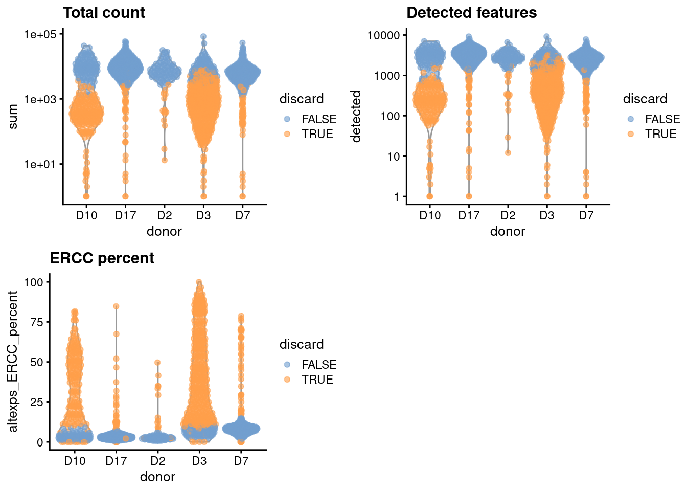
We compute the median and MAD while blocking on the donor; for donors where the assumption of a majority of high-quality cells seems to be violated (Figure \@ref(fig:unref-grun-qc-dist)), we compute an appropriate threshold using the other donors as specified in the `subset=` argument. ```r library(scater) stats <- perCellQCMetrics(sce.grun) qc <- quickPerCellQC(stats, percent_subsets="altexps_ERCC_percent", batch=sce.grun$donor, subset=sce.grun$donor %in% c("D17", "D7", "D2")) sce.grun <- sce.grun[,!qc$discard] ``` ```r colData(unfiltered) <- cbind(colData(unfiltered), stats) unfiltered$discard <- qc$discard gridExtra::grid.arrange( plotColData(unfiltered, x="donor", y="sum", colour_by="discard") + scale_y_log10() + ggtitle("Total count"), plotColData(unfiltered, x="donor", y="detected", colour_by="discard") + scale_y_log10() + ggtitle("Detected features"), plotColData(unfiltered, x="donor", y="altexps_ERCC_percent", colour_by="discard") + ggtitle("ERCC percent"), ncol=2 ) ```
Distribution of each QC metric across cells from each donor of the Grun pancreas dataset. Each point represents a cell and is colored according to whether that cell was discarded.

(\#fig:unref-grun-qc-dist)Distribution of each QC metric across cells from each donor of the Grun pancreas dataset. Each point represents a cell and is colored according to whether that cell was discarded.

```r colSums(as.matrix(qc), na.rm=TRUE) ``` ``` ## low_lib_size low_n_features high_altexps_ERCC_percent ## 450 512 606 ## discard ## 665 ``` ## Normalization ```r library(scran) set.seed(1000) # for irlba. clusters <- quickCluster(sce.grun) sce.grun <- computeSumFactors(sce.grun, clusters=clusters) sce.grun <- logNormCounts(sce.grun) ``` ```r summary(sizeFactors(sce.grun)) ``` ``` ## Min. 1st Qu. Median Mean 3rd Qu. Max. ## 0.099 0.511 0.796 1.000 1.231 8.838 ``` ```r plot(librarySizeFactors(sce.grun), sizeFactors(sce.grun), pch=16, xlab="Library size factors", ylab="Deconvolution factors", log="xy") ```
Relationship between the library size factors and the deconvolution size factors in the Grun pancreas dataset.

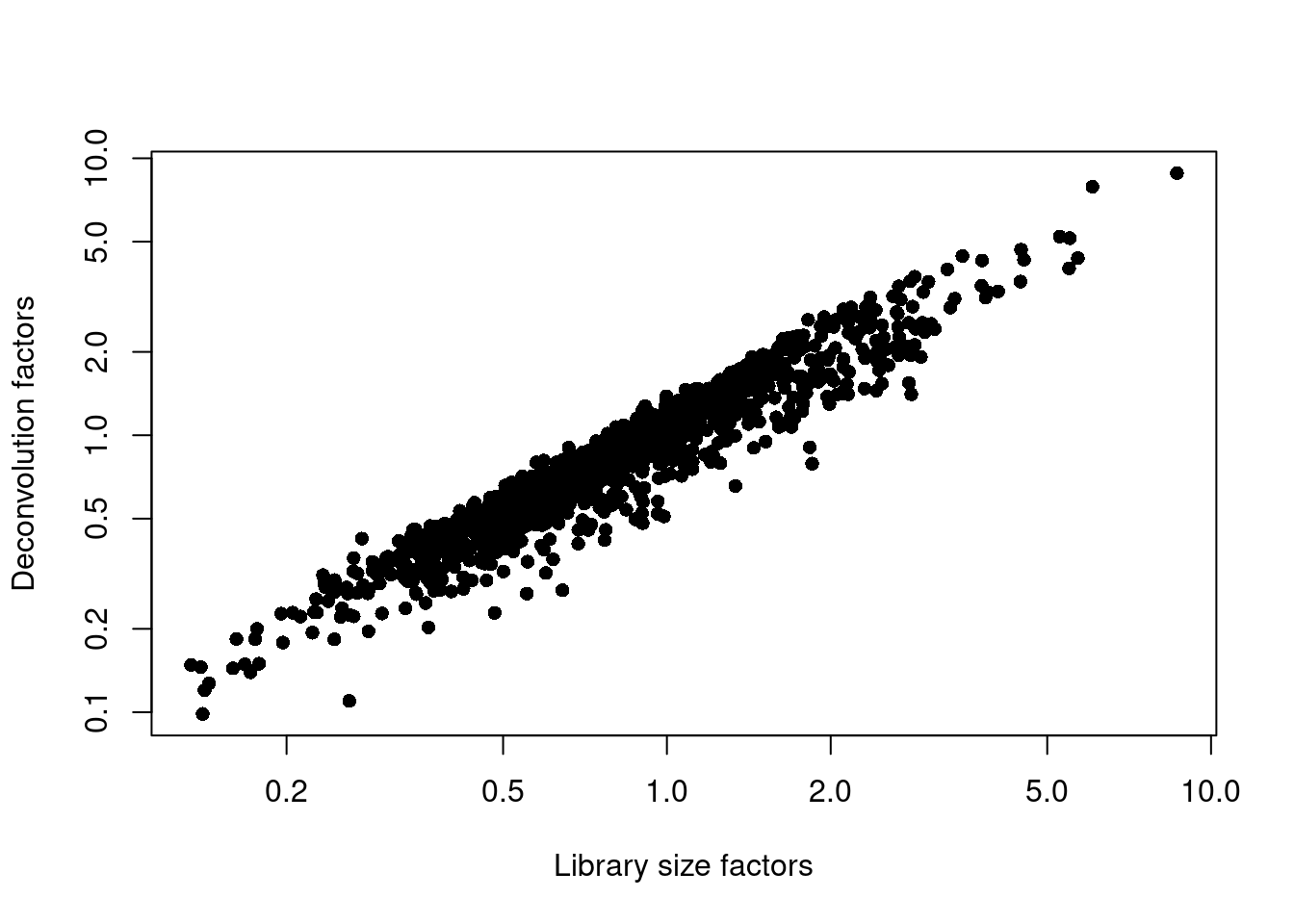
(\#fig:unref-grun-norm)Relationship between the library size factors and the deconvolution size factors in the Grun pancreas dataset.

## Variance modelling 
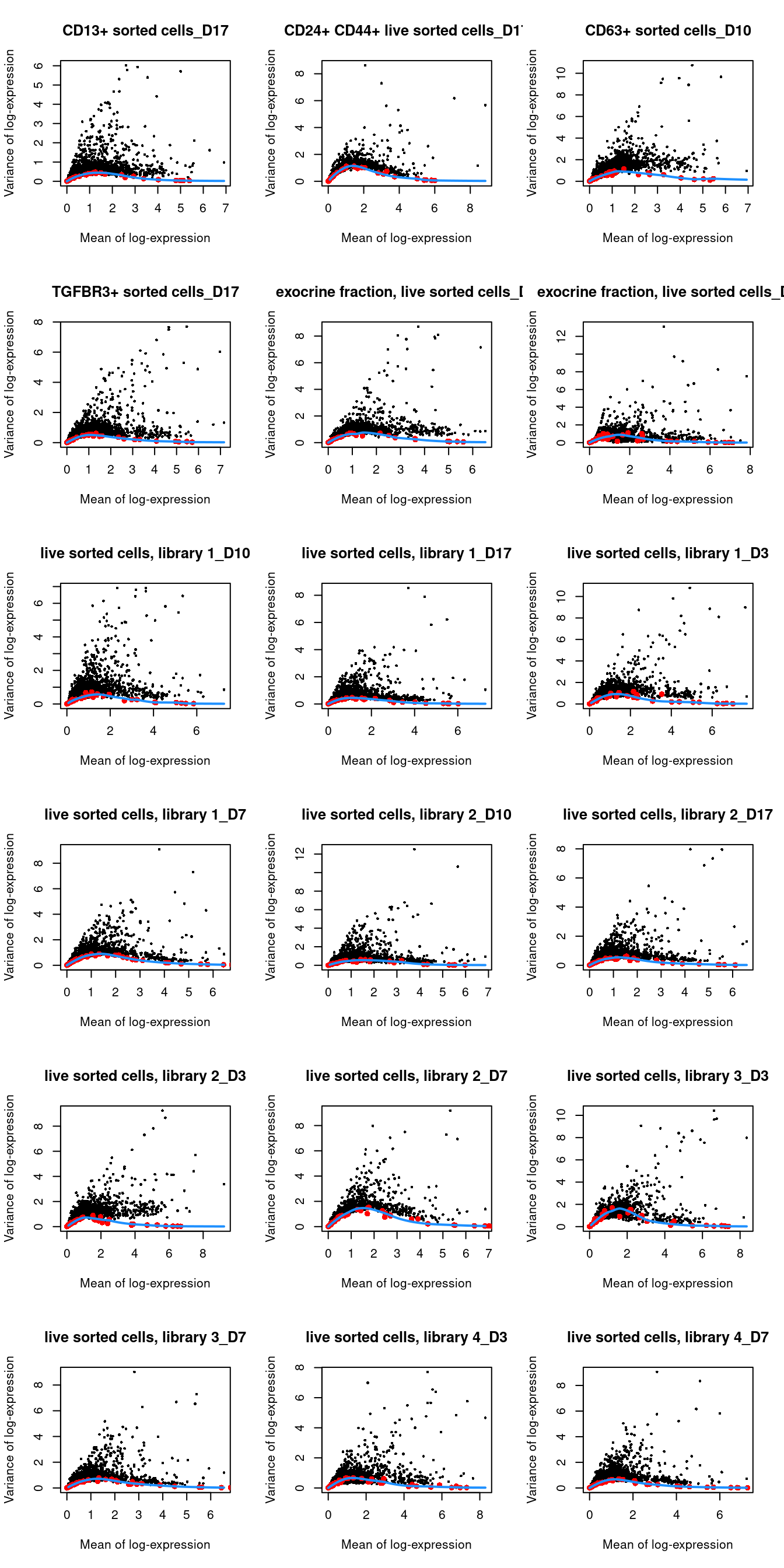
We block on a combined plate and donor factor. ```r block <- paste0(sce.grun$sample, "_", sce.grun$donor) dec.grun <- modelGeneVarWithSpikes(sce.grun, spikes="ERCC", block=block) top.grun <- getTopHVGs(dec.grun, prop=0.1) ``` We examine the number of cells in each level of the blocking factor. ```r table(block) ``` ``` ## block ## CD13+ sorted cells_D17 CD24+ CD44+ live sorted cells_D17 ## 86 87 ## CD63+ sorted cells_D10 TGFBR3+ sorted cells_D17 ## 41 90 ## exocrine fraction, live sorted cells_D2 exocrine fraction, live sorted cells_D3 ## 82 7 ## live sorted cells, library 1_D10 live sorted cells, library 1_D17 ## 33 88 ## live sorted cells, library 1_D3 live sorted cells, library 1_D7 ## 24 85 ## live sorted cells, library 2_D10 live sorted cells, library 2_D17 ## 35 83 ## live sorted cells, library 2_D3 live sorted cells, library 2_D7 ## 27 84 ## live sorted cells, library 3_D3 live sorted cells, library 3_D7 ## 16 83 ## live sorted cells, library 4_D3 live sorted cells, library 4_D7 ## 29 83 ``` ```r par(mfrow=c(6,3)) blocked.stats <- dec.grun$per.block for (i in colnames(blocked.stats)) { current <- blocked.stats[[i]] plot(current$mean, current$total, main=i, pch=16, cex=0.5, xlab="Mean of log-expression", ylab="Variance of log-expression") curfit <- metadata(current) points(curfit$mean, curfit$var, col="red", pch=16) curve(curfit$trend(x), col='dodgerblue', add=TRUE, lwd=2) } ```
Per-gene variance as a function of the mean for the log-expression values in the Grun pancreas dataset. Each point represents a gene (black) with the mean-variance trend (blue) fitted to the spike-in transcripts (red) separately for each donor.

(\#fig:unref-416b-variance)Per-gene variance as a function of the mean for the log-expression values in the Grun pancreas dataset. Each point represents a gene (black) with the mean-variance trend (blue) fitted to the spike-in transcripts (red) separately for each donor.

## Data integration ```r library(batchelor) set.seed(1001010) merged.grun <- fastMNN(sce.grun, subset.row=top.grun, batch=sce.grun$donor) ``` ```r metadata(merged.grun)$merge.info$lost.var ``` ``` ## D10 D17 D2 D3 D7 ## [1,] 0.030626 0.032123 0.000000 0.00000 0.00000 ## [2,] 0.007151 0.011372 0.036091 0.00000 0.00000 ## [3,] 0.003905 0.005135 0.007729 0.05239 0.00000 ## [4,] 0.011862 0.014643 0.013594 0.01235 0.05387 ``` ## Dimensionality reduction ```r set.seed(100111) merged.grun <- runTSNE(merged.grun, dimred="corrected") ``` ## Clustering ```r snn.gr <- buildSNNGraph(merged.grun, use.dimred="corrected") colLabels(merged.grun) <- factor(igraph::cluster_walktrap(snn.gr)$membership) ``` ```r table(Cluster=colLabels(merged.grun), Donor=merged.grun$batch) ``` ``` ## Donor ## Cluster D10 D17 D2 D3 D7 ## 1 32 70 31 80 28 ## 2 14 34 3 2 67 ## 3 12 71 31 2 71 ## 4 5 4 2 4 2 ## 5 11 119 0 0 55 ## 6 2 8 3 3 6 ## 7 3 40 0 0 10 ## 8 1 9 0 0 7 ## 9 15 36 12 11 45 ## 10 5 13 0 0 10 ## 11 4 13 0 0 1 ## 12 5 17 0 1 33 ``` ```r gridExtra::grid.arrange( plotTSNE(merged.grun, colour_by="label"), plotTSNE(merged.grun, colour_by="batch"), ncol=2 ) ```
Obligatory $t$-SNE plots of the Grun pancreas dataset. Each point represents a cell that is colored by cluster (left) or batch (right).

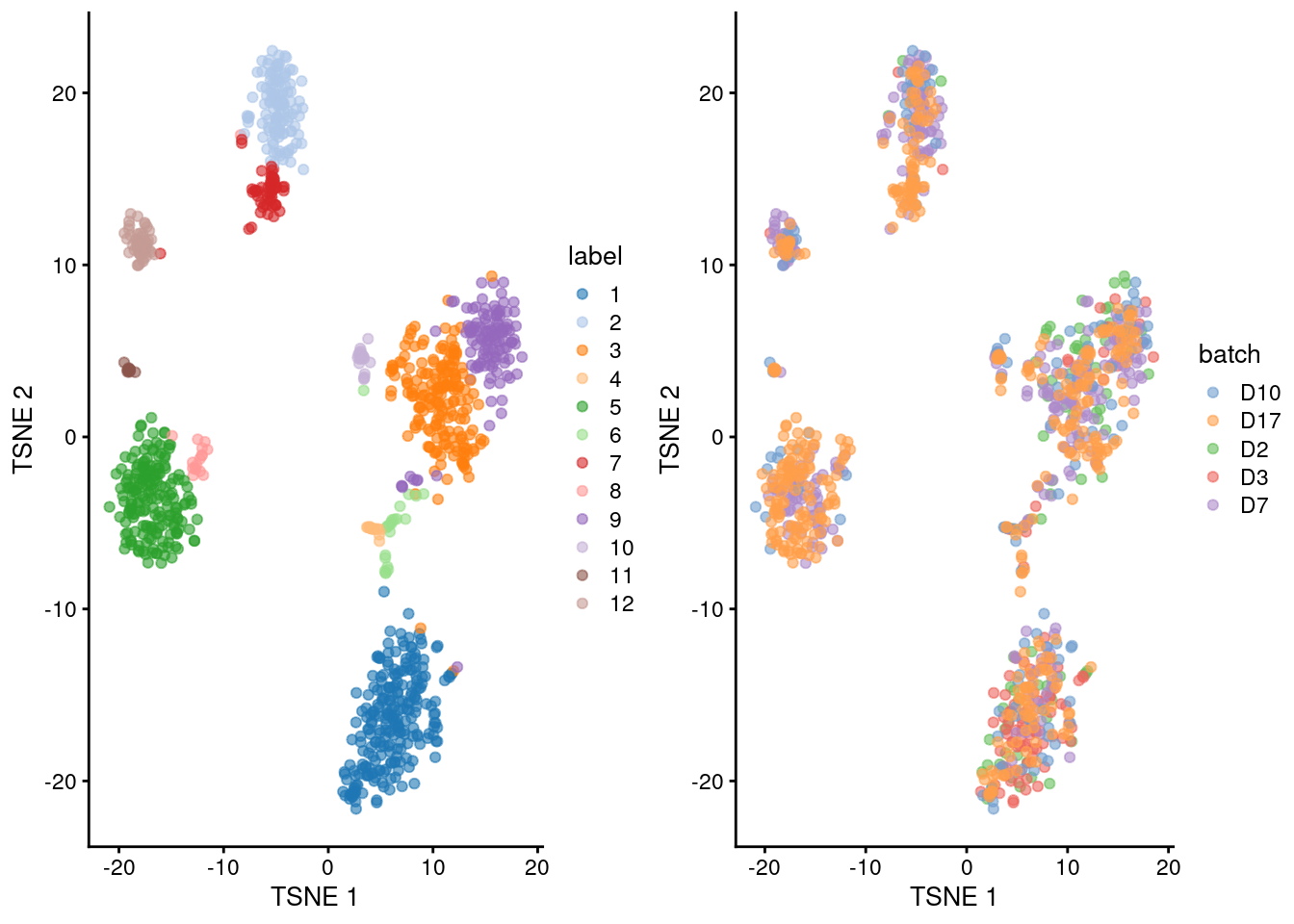
(\#fig:unref-grun-tsne)Obligatory $t$-SNE plots of the Grun pancreas dataset. Each point represents a cell that is colored by cluster (left) or batch (right).

## Session Info {-}
``` R version 4.0.4 (2021-02-15) Platform: x86_64-pc-linux-gnu (64-bit) Running under: Ubuntu 20.04.2 LTS Matrix products: default BLAS: /home/biocbuild/bbs-3.12-books/R/lib/libRblas.so LAPACK: /home/biocbuild/bbs-3.12-books/R/lib/libRlapack.so locale: [1] LC_CTYPE=en_US.UTF-8 LC_NUMERIC=C [3] LC_TIME=en_US.UTF-8 LC_COLLATE=C [5] LC_MONETARY=en_US.UTF-8 LC_MESSAGES=en_US.UTF-8 [7] LC_PAPER=en_US.UTF-8 LC_NAME=C [9] LC_ADDRESS=C LC_TELEPHONE=C [11] LC_MEASUREMENT=en_US.UTF-8 LC_IDENTIFICATION=C attached base packages: [1] parallel stats4 stats graphics grDevices utils datasets [8] methods base other attached packages: [1] batchelor_1.6.2 scran_1.18.5 [3] scater_1.18.6 ggplot2_3.3.3 [5] org.Hs.eg.db_3.12.0 AnnotationDbi_1.52.0 [7] scRNAseq_2.4.0 SingleCellExperiment_1.12.0 [9] SummarizedExperiment_1.20.0 Biobase_2.50.0 [11] GenomicRanges_1.42.0 GenomeInfoDb_1.26.4 [13] IRanges_2.24.1 S4Vectors_0.28.1 [15] BiocGenerics_0.36.0 MatrixGenerics_1.2.1 [17] matrixStats_0.58.0 BiocStyle_2.18.1 [19] rebook_1.0.0 loaded via a namespace (and not attached): [1] AnnotationHub_2.22.0 BiocFileCache_1.14.0 [3] igraph_1.2.6 lazyeval_0.2.2 [5] BiocParallel_1.24.1 digest_0.6.27 [7] ensembldb_2.14.0 htmltools_0.5.1.1 [9] viridis_0.5.1 fansi_0.4.2 [11] magrittr_2.0.1 memoise_2.0.0 [13] limma_3.46.0 Biostrings_2.58.0 [15] askpass_1.1 prettyunits_1.1.1 [17] colorspace_2.0-0 blob_1.2.1 [19] rappdirs_0.3.3 xfun_0.22 [21] dplyr_1.0.5 callr_3.5.1 [23] crayon_1.4.1 RCurl_1.98-1.3 [25] jsonlite_1.7.2 graph_1.68.0 [27] glue_1.4.2 gtable_0.3.0 [29] zlibbioc_1.36.0 XVector_0.30.0 [31] DelayedArray_0.16.2 BiocSingular_1.6.0 [33] scales_1.1.1 edgeR_3.32.1 [35] DBI_1.1.1 Rcpp_1.0.6 [37] viridisLite_0.3.0 xtable_1.8-4 [39] progress_1.2.2 dqrng_0.2.1 [41] bit_4.0.4 rsvd_1.0.3 [43] ResidualMatrix_1.0.0 httr_1.4.2 [45] ellipsis_0.3.1 pkgconfig_2.0.3 [47] XML_3.99-0.6 farver_2.1.0 [49] scuttle_1.0.4 CodeDepends_0.6.5 [51] sass_0.3.1 dbplyr_2.1.0 [53] locfit_1.5-9.4 utf8_1.2.1 [55] tidyselect_1.1.0 labeling_0.4.2 [57] rlang_0.4.10 later_1.1.0.1 [59] munsell_0.5.0 BiocVersion_3.12.0 [61] tools_4.0.4 cachem_1.0.4 [63] generics_0.1.0 RSQLite_2.2.4 [65] ExperimentHub_1.16.0 evaluate_0.14 [67] stringr_1.4.0 fastmap_1.1.0 [69] yaml_2.2.1 processx_3.4.5 [71] knitr_1.31 bit64_4.0.5 [73] purrr_0.3.4 AnnotationFilter_1.14.0 [75] sparseMatrixStats_1.2.1 mime_0.10 [77] xml2_1.3.2 biomaRt_2.46.3 [79] compiler_4.0.4 beeswarm_0.3.1 [81] curl_4.3 interactiveDisplayBase_1.28.0 [83] statmod_1.4.35 tibble_3.1.0 [85] bslib_0.2.4 stringi_1.5.3 [87] highr_0.8 ps_1.6.0 [89] GenomicFeatures_1.42.2 lattice_0.20-41 [91] bluster_1.0.0 ProtGenerics_1.22.0 [93] Matrix_1.3-2 vctrs_0.3.6 [95] pillar_1.5.1 lifecycle_1.0.0 [97] BiocManager_1.30.10 jquerylib_0.1.3 [99] BiocNeighbors_1.8.2 cowplot_1.1.1 [101] bitops_1.0-6 irlba_2.3.3 [103] httpuv_1.5.5 rtracklayer_1.50.0 [105] R6_2.5.0 bookdown_0.21 [107] promises_1.2.0.1 gridExtra_2.3 [109] vipor_0.4.5 codetools_0.2-18 [111] assertthat_0.2.1 openssl_1.4.3 [113] withr_2.4.1 GenomicAlignments_1.26.0 [115] Rsamtools_2.6.0 GenomeInfoDbData_1.2.4 [117] hms_1.0.0 grid_4.0.4 [119] beachmat_2.6.4 rmarkdown_2.7 [121] DelayedMatrixStats_1.12.3 Rtsne_0.15 [123] shiny_1.6.0 ggbeeswarm_0.6.0 ```